On writing GeoServer SLDs (part II)

In the last post I was writing about how to generate fixed random colors for GeoServer SLD files using the md5 function. The approach described there makes it easy to manage those cases where you need to maintain styles for a large number of layers with a large number of different classes or groups for features that needed to be styled categorically, with different colors. And in cases you don’t really care about the exact colorspace used. This time around I’m going to look how to make this random-color SLD style reusable for different layer properties.

GeoServer comes packed with some really neat capabilities when it comes to layer configuration. One of them is SQL view parameters. These are essentially key-value pair encode parameters that are passed to the underlying SQL view DB query during WMS / WFS get* operations. As the use of SQL view parameters is possibly a risk of SQL injection attacks these should be used carefully and harness the correct parameter validation rules aswell.

SQL view parameters essentially allow to do the same things that the cql_filter does but they also enable us to construct more elaborate DB queries. The way GeoServer composes a query to the DB is in general terms in the line of:

select
    this, that, whatever, that is, needed
from (
    <your layer query>
) as vtable
where
    <geom filter and cql_filter>

which in most cases is all you need to fetch data for (and possibly style) your layer. But it makes it fairly tedious for the database if for example your original query consists of multiple joins or (subquery) aggregates. By using view parameters we can help the database in the query execution by filtering out the unneeded rows already beforehand.

To illustrate this let’s use the address data from the Estonian Land Board’s ADS system. We’ll download the csv file published under the title Jõusolevad aadressiobjektid koos aadressidega (i.e. active address objects with addresses) from

https://xgis.maaamet.ee/adsavalik/extracts

If you’re following along word by word then out of the two options numbered 1 on the extracts download page choose the one with larger file size - the smaller is only for the city of Tallinn.

Unzip the file, create a table in your local PostgreSQL database as

create table public.address_object
(
    adob_id bigint,
    ads_oid character varying(20),
    adob_liik character varying(2),
    orig_tunnus character varying(50),
    etak_id bigint,
    ads_kehtiv timestamp without time zone,
    un_tunnus smallint,
    hoone_oid character varying(20),
    adr_id bigint,
    koodaadress character varying(50),
    taisaadress character varying(500),
    lahiaadress character varying(150),
    aadr_olek character varying(1),
    viitepunkt_x numeric(10,2),
    viitepunkt_y numeric(10,2),
    tase1_kood character varying(4),
    tase1_nimetus character varying(250),
    tase1_nimetus_liigiga character varying(250),
    tase2_kood character varying(4),
    tase2_nimetus character varying(250),
    tase2_nimetus_liigiga character varying(250),
    tase3_kood character varying(4),
    tase3_nimetus character varying(250),
    tase3_nimetus_liigiga character varying(250),
    tase4_kood character varying(4),
    tase4_nimetus character varying(250),
    tase4_nimetus_liigiga character varying(250),
    tase5_kood character varying(4),
    tase5_nimetus character varying(250),
    tase5_nimetus_liigiga character varying(250),
    tase6_kood character varying(4),
    tase6_nimetus character varying(250),
    tase6_nimetus_liigiga character varying(250),
    tase7_kood character varying(4),
    tase7_nimetus character varying(250),
    tase7_nimetus_liigiga character varying(250),
    tase8_kood character varying(4),
    tase8_nimetus character varying(250),
    tase8_nimetus_liigiga character varying(250)
);

and then import the csv with psql (mind the csv filename, could be different :))

~/data/tmp$ psql -h localhost -d postgres -U postgres -c "copy public.address_object (adob_id,ads_oid,adob_liik,orig_tunnus,etak_id,ads_kehtiv,un_tunnus,hoone_oid,adr_id,koodaadress,taisaadress,lahiaadress,aadr_olek,viitepunkt_x,viitepunkt_y,tase1_kood,tase1_nimetus,tase1_nimetus_liigiga,tase2_kood,tase2_nimetus,tase2_nimetus_liigiga,tase3_kood,tase3_nimetus,tase3_nimetus_liigiga,tase4_kood,tase4_nimetus,tase4_nimetus_liigiga,tase5_kood,tase5_nimetus,tase5_nimetus_liigiga,tase6_kood,tase6_nimetus,tase6_nimetus_liigiga,tase7_kood,tase7_nimetus,tase7_nimetus_liigiga,tase8_kood,tase8_nimetus,tase8_nimetus_liigiga) FROM '~/data/tmp/1_7042020_11120_1.csv' delimiter ';' null '""' csv header encoding 'WIN1257'"

As we’re already at it in the DB let’s set up some indexes. Let’s add them to akood (settlement identifier) and okood (municipality identifier) to the public.asustusyksus table that we imported in the previous SLD-post

create index idx__asustusyksus__okood on public.asustusyksus using btree(okood);
create index idx__asustusyksus__akood on public.asustusyksus using btree(akood);

And in addition do some data-fixing in the newly imported public.address_object table. We’ll do this to make public.asustusyksus and our new shining address objects table public.address_object easily joinable.

-- update admin level 1 code for address to match that of admin-division: must be 0-padded 4 chars
update public.address_object set tase1_kood = lpad(tase1_kood, 4, '0') where tase1_kood != '' ;

-- update admin level 2 code for address to match that of admin-division: must be 0-padded 4 chars
update public.address_object set tase2_kood = lpad(tase2_kood, 4, '0') where tase2_kood != '' ;

-- update level 3 code to 0-padded 4-char level 2 code if missing
-- if the municipality and settlement units have the same name and same borders
-- these settlements will not be recorded in the ADS dataset.
update public.address_object set tase3_kood = lpad(tase2_kood, 4, '0') where tase3_kood = '' and adob_liik != all(array['MK', 'OV']);

-- and add indexes here aswell
create index idx__address_object__tase1_kood on public.address_object using btree(tase1_kood);
create index idx__address_object__tase2_kood on public.address_object using btree(tase2_kood);
create index idx__address_object__tase3_kood on public.address_object using btree(tase3_kood);

Right. Now as a testcase for viewparams let’s query for the amount of EE (“residential”), ME (“non-residential”) and CU (“cadastral unit”) address objects per settlement unit:

select
    ay.* , foo.count
from
    public.asustusyksus ay, (
        select
            tase3_kood, count(1)
        from
            public.address_object ao
        where
            ao.adob_liik = any(array['EE','ME','CU'])
        group by tase3_kood
    ) foo
where
    foo.tase3_kood = ay.akood

In my local database this query retuns all settlement unit data from public.asustusyksus and a count of address objects with types EE, ME, CU in roughly 1.5 seconds. Now if I wanted to restrict the returned rows for example by a municipality identifier the most obvious place for it would be in the subquery foo where clause instead of the outer where. We can easily try this out.

select
    ay.* , foo.count
from
    public.asustusyksus ay, (
        select
            tase3_kood, count(1)
        from
            public.address_object ao
        where
            ao.adob_liik = any(array['EE','ME','CU']) and
            ao.tase2_kood = '0615' -- Põhja-Sakala vald
        group by tase3_kood
    ) foo
where
    foo.tase3_kood = ay.akood

Returns roughly in 90ms. While simulating the kind of query (but not exactly) that goes out by default from GeoServer if we use a cql_filter

select
    *
from (
    select
        ay.* , foo.count
    from
        public.asustusyksus ay, (
            select
                tase3_kood, count(1)
            from
                public.address_object ao
            where
                ao.adob_liik = any(array['EE','ME','CU'])
            group by tase3_kood
        ) foo
    where
        foo.tase3_kood = ay.akood
) bar
where
    bar.okood = '0615' -- Põhja-Sakala vald

This returns the same result as before, only this time in roughly 600ms. So as we can see there are cases when it makes sense to use viewparams to speed up queryies from GeoServer to the undelying database.

But the reason we’re interested in viewparams in this case is that it’s not only column values that can be parameterized but also column names. Going back to the query used in the previous post it is possible to parameterize the column name that we’ll be sending into the md5 function for random-color calculation.

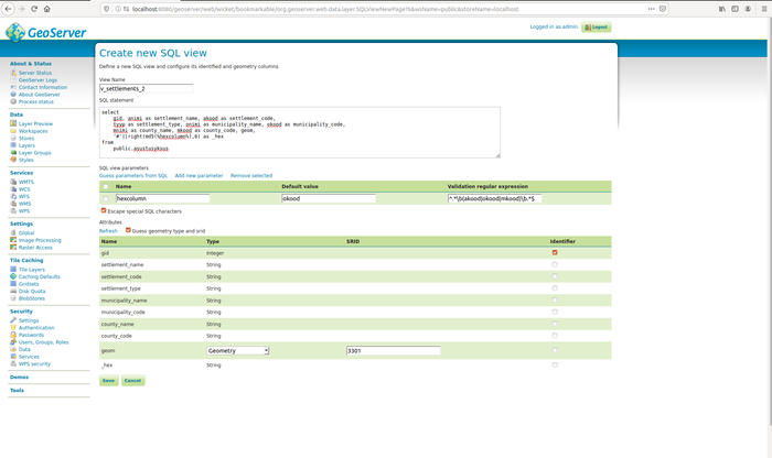
So let’s add a new SQL view based layer. The SQL is essentially the same as last time around only this time let’s parameterize the input column name to the md5 hash-function:

select
    gid, animi as settlement_name, akood as settlement_code,
    tyyp as settlement_type, onimi as municipality_name, okood as municipality_code,  
    mnimi as county_name, mkood as county_code, geom,
    '#'||right(md5(%hexcolumn%),6) as _hex
from
    public.asustusyksus

with a default value of onimi for viewparam called hexcolumn and ^.*\b(animi|onimi|mnimi)\b.*$ as the regexp validator to guard this viewparam. With this we’re narrowing the possible inputs for our viewparam down to animi, onimi or mnimi. And GeoServer will complain if you try to pass anything else as the parameter value.

Add the same hex-based style we created before (public:area.autostyle.hex) as the default style and publish the layer. Now browsing the layer preview at your local GeoServer should yield the same colors and style as the layer published before which is good. This is because we’re using the same default column name in hex-calculation. But now we have an easy possibility to change the column by which the random-color-calculation takes place. For example, if we wanted to color the settlement units by the 1st level admin unit they belong to we simply need to add

&viewparams=hexcolumn:mnimi

to the getmap operation queryparams and behold

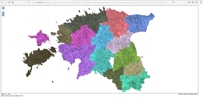
or

&viewparams=hexcolumn:animi

to produce a proper patchwork quilt

That’s it for this time. Thanks for following through and if you’re interested then stay tuned for at least one more episode on my encounters with SLD which will cover the topic of producing discrete and interpolated color thematic maps with a single SLD.

As previously all required $GEOSERVER_DATA_DIR/workspaces files to set this up locally are available at this github repo under CC-BY-SA 4.0